Petroleum Engineering Equations & Formulas Part -2

Compressibility of oil

Pressure depletion in the reservoir can normally be assumed to be isothermal, such that the isothermal compressibility is defined as the fractional change in volume per unit change in pressure:

       c = -(1/V) DOT dV/dP  [psi-1] or [bar-1]

       Where:

       dV : derivative of volume
       dP : derivative of pressure
       V  : volume

Generating Expecting Curves TO BE COMPLETED

STOIIP is a term which normalises volumes of oil contained under high pressure and temperature in the subsurface conditions.

GIIP is the equivilant expression for gas initially in place.

GRV is the Gross Rock Volume of the hydrocarbon-bearing interval and is the priduct of the area (A) containing hydrocarbons and interval thickness (H).
      STOIIP = GRV * (N/V) * Φ * So * (1/Bo) [stb]

      GIIP = GRV * (N/V) * Φ * Sg * (1/Bg) [stb]

      GRV = A * H

      Ultimate recovery = HCIIP * Recovery Factor [stb] or [scf]

      Reserves = Ultimate Recovery - Cumulative Production [stb] or [scf]





Fluid Flow near the Wellbore

The difference between the following wellbore pressure (Pwf) and the average reservoir pressure ( P) is the pressure drawdown (ΔPDD).
       Pressure drawdown ΔPDD = P - Pwf [psi] or [bar]

       Where:

       P is Reservoir pressure
       P wf is Flowing wellbore pressure
            

The relationship between the floarate (Q) towards the well and the pressure drawdown is approximately linear, and is defined by the productivity index (PI)
       Productivity Index PI = Q/ΔPDD [bbl/d/psi] or [m3/d/bar]
            

The flowrate of oil into the wellbore is also influenced by the reservoir properties of permeability(k) and the reservoir thickness(h), by the oil properties viscosity(μ) and formation volume factor (Bo) and by any change in the resistance to flow near the wellbore whch is represented bu the dimensionless term called skin (S). For semi-steady state flow behaviour abd radial inflow for the oil into a vertical wellbore is represented by equation 3:



Ultimate Recovery 

In estimating the ultimate recovery (UR) for an oil reservoir, one would need to use the following:
      UR = Area * thickness * (N/G) * Φ * So * (1/Bo) * RF

      Where:

      Φ is porosity
      So is the oil saturation in the pore space
      Bo is the formation volume factor of the oil
      RF is the recovery factor



Oil & gas volumes

STOIIP is a term which normalises volumes of oil contained under high pressure and temperature in the subsurface conditions.

GIIP is the equivilant expression for gas initially in place.

GRV is the Gross Rock Volume of the hydrocarbon-bearing interval and is the priduct of the area (A) containing hydrocarbons and interval thickness (H).
      STOIIP = GRV * (N/V) * Φ * So * (1/Bo) [stb]

      GIIP = GRV * (N/V) * Φ * Sg * (1/Bg) [stb]

      GRV = A * H

      Ultimate recovery = HCIIP * Recovery Factor [stb] or [scf]

      Reserves = Ultimate Recovery - Cumulative Production [stb] or [scf]


Recovery Factory


The recovery factor(RF) defines the relationship between the hydrocarbons initially in place (HCIIP) and the ultimate recovery for the field.
       UR = HCIIP * RF [stb] or [scf]

       R = UR - CP [stb] or [scf]

       Where:

       UR is Ultimate recovery
       RF is Recovery factor
       R  is Reserves
       CP is Cumulative Production


SolutionGas Drive : Water cut


Commonly the water cut remains small in solution gas drive reservoirs, assuming that there is little pressure support provided by the underlying aquifer. Water cut is also referred to as BS&W(Base, Sediment & water) and is defined as:
      Water cut (BS&W) = (water production / oil plus water production) * 100(%)

Petroleum Engineering Equations & Formulas Part -1

Oil density

Oil density at surface conditions is commonly quoted in °API.

       API = 141.5/γo-131.5

       Where: γo is the specific gravity of oil (relative to water = 1, measured at STP).
            

The downhole density of oil (at reservoir conditions) can be calculated from the surface density equation using:

       ρorc * Bo = ρo + Rs * ρg

       Where:

       ρorc : is oil density at reservoir conditions 

       Bo   : is the oil formation volume factor     

       ρo   : is oil density at standard conditions  

       Rs   : is the solution gas : oil ratio 

Fluid Pressure

Assuming a normal pressure regime, at a given depth below ground level, a certain pressure must exist which just balances the overburden pressure (OBP) due to the weight of rock (which forms a matrix) and fluid (which fills the matrix) overlying this point. The overburden pressure is in fact balanced by a combination of the fluid pressure in the pore space (FP) and the sress between the rock grains of the matrix (σg).

Formula:

       OBP = FP + σg

       Where:

       σg: is the stress between the rock grains of the matrix

       FP: is the fluid pressure in the pore space.

Porosity

Reservoir porosity can be measured directly from core samples or indirectly using logs. Logging is the most common method employed. The formation density log is the main tool for ensuring porosity. The tool is constructed so that medium energy gamma rays are directed from a radioactive source into the formation. These rays react with the formation by a process know as Compton scattering. Gamma rays lose energy each time they collide with an electron. The number of gamma rays reaching detectors in the tool is inversely proportional to the number of electrons in the formation which is related to the formation bulk density. A low gamma count implies a high electron (and bulk) density and therefore a low porosity

The bulk density measured by the logging tool is the weighted average of the rock matrix and fluid densities so that:
       ρb = ρflΦ + ρma(1-Φ)

       Where:

       ρb : is the formation bulk density (read from the density log)

       ρma: is the matrix density

       ρfl: is the fluid density

            

Porosity (Φ) is:
       Φ = (ρma - ρb) / (ρma - ρfl)

Hydrocarbon Saturation

       Ct = SwnΦm Cw

       Where:

       Ct: is the conductivity

       Cw: is the pore water conductivity

       Sw: is the water saturation

       n : is the saturation exponent

       m : is the cementation exponent

            

In pratice logging tools are often used to measure the resistivity of the formation rather than the conductivity and therefore the above equation is more commonly inverted and expressed as:
       Rt = Sw-nΦ-mRw

       Where:

       Rt: is the formation resistivity (ohm.m)

       Sw: is the water saturation (fraction)

       Φ : is porosity(fraction)

       Rw: is the water resistivity (ohm.m)

       m : is the cementation exponent

       n : is the saturation exponent
            

In a large ange of reservoirs the saturation and cememntation exponents can be taken as m=n=2. The remaining unknown is the water saturation and the equation can be rearranged so that:
            Sw = n√((Rw)/(ΦmRt))

                and hydrocarbon saturation (fraction)

            Sh= 1 - Sw

Diffusivity Equation & Radius of Investigate (ROI)

Radius of Investigate : 2Examples

Equations for Single-Phase Porous Media Flow

Equations for Single-Phase Porous Media Flow

• Introduction : 

The flow of a single, compressible fluid through porous, permeable rock can be described using a partial differential equation known as the diffusivity equation. Modified forms of the diffusivity equation can be used to describe gas flow. A similar equation can be derived for multiphase flow as well, and that equation is the basis for reservoir simulation. Clearly, the diffusivity equation is at the very heart of reservoir engineering and an intuitive understanding of this equation is essential to all who would do reservoir engineering.

• The Conservation Equation : 

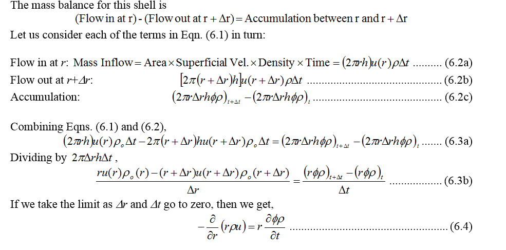
Many physical systems – ranging from solar collectors to river deltas to flow in reservoirs – can be analyzed using the principle of conservation. This principle is closely related to the idea of a control volume in thermodynamics; it is based on the idea that the amount of “stuff” (energy, mass, whatever) entering, leaving, created, and destroyed in a given volume must be balanced. We will derive the conservation equation for a radial flow geometry, because this geometry is especially useful for well testing and inflow analysis. We could do it for any geometry we chose. 

Consider a cylindrical shell of radius r and thickness Dr (Figure 6.1). 

Equation (6.4) is the conservation equation in radial coordinates. It states that the sum of the partial differential derivatives in r and t is zero. This is also known as a divergence equation; all conservation equations (for any quantity, in any coordinate system) can be expressed in a form very similar to Equation 6.4. 

This equation must be manipulated further to be useful: it includes dependent variables r, f, and u, whereas we really want an equation in p only. We will use constitutive equations for these quantities to get the desired equation.

• Use of Darcy’s Law in the Conservation Equation

• The Case of Small and Constant Compressibility

• The Linearized Diffusivity Equation

Although Equation (6.10) is in pressure, it is nonlinear. It is very difficult to solve nonlinear partial differential equations, and we therefore seek a simplified, linear form to work with. The nonlinearity comes from two different sources.

• Dimensionless Variables

We used the concept of a dimensionless variable when we discussed the skin factor. We will extend that discussion now to better understand the linearized diffusivity equation. It seems sensible to make radius dimensionless on the wellbore radius :

• Other Coordinate Systems and Notation

• Discussion

Assumptions The steps and assumptions used to derive the linearized diffusivity equation are summarized in Table 6.1, below:

The assumptions are very important to be familiar with. Study this table! In particular, consider the following:

PE Petroleum Engineering Syllabus

PE Petroleum Engineering Syllabus 

1. Linear Algebra: Matrix algebra, Systems of linear equations, Eigen values and eigenvectors.

2. Calculus: Functions of single variable, Limit, continuity and differentiability, Taylor series,

Mean value theorems, Evaluation of definite and improper integrals, Partial derivatives, Total

derivative, Maxima and minima, Gradient, Divergence and Curl, Vector identities, Directional

derivatives, Line, Surface and Volume integrals, Stokes, Gauss and Green’s theorems.

3. Differential equations: First order equations (linear and nonlinear), Higher order linear

differential equations with constant coefficients, Cauchy’s and Euler’s equations, Initial and

boundary value problems, Laplace transforms, Solutions of one dimensional heat and wave

equations and Laplace equation.

4. Complex variables: Complex number, polar form of complex number, triangle inequality.

5. Probability and Statistics: Definitions of probability and sampling theorems, Conditional

probability, Mean, median, mode and standard deviation, Random variables, Poisson, Normal

and Binomial distributions, Linear regression analysis.

6. Numerical Methods: Numerical solutions of linear and non-linear algebraic equations.

Integration by trapezoidal and Simpson’s rule. Single and multi-step methods for numerical

solution of differential equations.

7. Petroleum Exploration: Classification and description of some common rocks with special

reference to clastic and nonclastic reservoir rocks. Origin, migration and accumulation of

Petroleum. Petroleum exploration methods.

8. Oil and Gas Well Drilling Technology: Well planning. Drilling method. Drilling rigs Rig

operating systems. Drilling fluids function and properties. Drilling fluid maintenance

equipment. Oil & gas well cementing operations. Drill bit types and their applications. Drill

string & Casing string function, operations, selection & design. Drilling problems, their control

& remedies. Directional drilling tools. Directional survey. Application of horizontal, multilateral,

extended reach, slim wells.

9. Reservoir Engineering: Petrophysical properties of reservoir rocks. Coring and core

analysis. Reservoir fluid properties. Phase behavior of hydrocarbon system. Flow of fluids

through porous media. Water and gas coning. Reservoir pressure measurements. Reservoir

drives, drive mechanics and recovery factors. Reserve estimation & techniques.

10. Petroleum Production Operations: Well equipments. Well completion techniques. Well

production problems and mitigation. Well servicing & Workover operations. Workover &

completion fluids. Formation damage. Well stimulation techniques. Artificial lift techniques.

Field processing of oil & gas. Storage and transportation of petroleum and petroleum

products. Metering and measurements oil & gas. Production system analysis & optimization.

Production testing. Multiphase flow in tubing and flow-lines. Nodal system analysis. Pressure

vessels, storage tanks, shell and tube heat exchangers, pumps and compressors, LNG value

chain.

11. Offshore Drilling and Production Practices: Offshore oil and gas operations & ocean

environment. Offshore fixed platforms, Offshore mobile units, Station keeping methods like

mooring & dynamic positioning system. Offshore drilling from fixed platform, jack-up, ships

and semi submersibles. Use of conductors and risers. Offshore well completion. Deep water

applications of subsea technology. Offshore production: Oil processing platforms, water

injection platforms, storage, SPM and SBM transportation and utilities. Deep water drilling rig.

Deep water production system. Emerging deep water technologies.

12. Petroleum Formation Evaluation: Evaluation of petrophysical of sub-surface formations:

Principles applications, advantages and disadvantages of SP, resistivity, radioactive, acoustic

logs and types of tools used. Evaluation of CBL/VDL, USIT, SFT, RFT. Production logging

tools, principles, limitations and applications. Special type of logging tools. Casing inspection

tools (principles, applications and limitations), Formations micro scanner (FMS), NMR logging

principles. Standard log interpretation methods. Cross-plotting methods.

13. Oil and Gas Well Testing: Diffusivity equation, derivation & solutions. Radius of

investigation. Principle of superposition. Horner’s approximation. Drill Stem Testing. Pressure

Transient Tests: Drawdown and build up-test analysis. Wellbore effects. Multilayer reservoirs.

Injection well testing. Multiple well testing. Interference testing, Pulse testing, well-test

analysis by use of type curves. Gas well testing.

14. Health Safety and Environment in Petroleum Industry: Health hazards in Petroleum

Industry: Toxicity, Physiological, Asphyxiation, respiratory and skin effect of petroleum

hydrocarbons, sour gases. Safety System: Manual & automatic shutdown system, blow down

systems. Gas detection system. Fire detection and suppression systems. Personal protection

system & measures. HSE Policies. Disaster & crisis management in Petroleum Industry.

Environment: Environment concepts, impact on eco-system, air, water and soil. The impact of

drilling & production operations on environment, Environmental transport of petroleum wastes.

Offshore environmental studies. Offshore oil spill and oil spill control. Waste treatment

methods.

15. Enhanced Oil Recovery Techniques: Basic principles and mechanism of EOR, Screening

of EOR process. Concept of pattern flooding, recovery efficiency, permeability heterogeneity.

Macroscopic and microscopic displacement efficiency. EOR methods: Chemical flooding,

Miscible flooding, Thermal recoveries (steam stimulation, hot water & steam flooding, in-situ

combustion), Microbial EOR.

16. Latest trends in Petroleum Engineering: Coal bed methane, shale gas, oil shale, gas

hydrate, and heavy oil.

Lesson 1 - Fundamentals of Reservoir Fluid Behavior

Lesson 1 -  Fundamentals of Reservoir Fluid Behavior

The objective of this chapter is to review the basic principles of reservoir fluid phase behavior and illustrate the use of phase diagrams in classifying types of reservoirs and the native hydrocarbon systems. 

• CLASSIFICATION OF RESERVOIRS AND RESERVOIR FLUID

Petroleum reservoirs are broadly classified as oil or gas reservoirs.These broad classifications are further subdivided depending on:

• The composition of the reservoir hydrocarbon mixture

• Initial reservoir pressure and temperature

• Pressure and temperature of the surface production

The conditions under which these phases exist are a matter of considerable practical importance. The experimental or the mathematical determinations of these conditions are conveniently expressed in different types of diagrams commonly called phase diagrams. One such diagram is called the pressure-temperature diagram.

Pressure-Temperature Diagram

Following figure 1.1 shows a typical pressure-temperature diagram of a multicomponent system with a specific overall composition. Although a different hydrocarbon system would have a different phase diagram, the general configuration is similar.

These multicomponent pressure-temperature diagrams are essentially used to:

• Classify reservoirs

• Classify the naturally occurring hydrocarbon systems

• Describe the phase behavior of the reservoir fluid

To fully understand the significance of the pressure-temperature diagrams, it is necessary to identify and define the following key points on these diagrams:

• Cricondentherm (Tct)—The Cricondentherm is defined as the maximum temperature above which liquid cannot be formed regardless of pressure (point E). The corresponding pressure is termed the Cricondentherm pressure pct.

• Cricondenbar (pcb)—The Cricondenbar is the maximum pressure above which no gas can be formed regardless of temperature (point D). The corresponding temperature is called the Cricondenbar temperature Tcb.

• Critical point—The critical point for a multicomponent mixture is referred to as the state of pressure and temperature at which all intensive properties of the gas and liquid phases are equal (point C). At the critical point, the corresponding pressure and temperature are called the critical pressure pc and critical temperature Tc of the mixture.

• Phase envelope (two-phase region)—The region enclosed by the bubble- point curve and the dew-point curve (line BCA), wherein gas and liquid coexist in equilibrium, is identified as the phase envelope of the hydrocarbon system.

• Quality lines—The dashed lines within the phase diagram are called quality lines. They describe the pressure and temperature conditions for equal volumes of liquids. Note that the quality lines converge at the critical point (point C).

• Bubble-point curve—The bubble-point curve (line BC) is defined as the line separating the liquid-phase region from the two-phase region.

• Dew-point curve—The dew-point curve (line AC) is defined as the line separating the vapor-phase region from the two-phase region.

Accordingly, reservoirs can be classified into basically two types. These are:

1. Oil reservoirs—If the reservoir temperature T is less than the critical temperature Tc of the reservoir fluid, the reservoir is classified as an oil reservoir.
2. Gas reservoirs—If the reservoir temperature is greater than the critical temperature of the hydrocarbon fluid, the reservoir is considered a gas reservoir.

Oil Reservoirs

Depending upon initial reservoir pressure pi, oil reservoirs can be sub classified  into the following categories:

1. Undersaturated oil reservoir. If the initial reservoir pressure pi (as represented by point 1 on Figure 1-1), is greater than the bubble-point pressure pb of the reservoir fluid, the reservoir is labeled an undersaturated oil reservoir.

2. Saturated oil reservoir. When the initial reservoir pressure is equal to the bubble-point pressure of the reservoir fluid, as shown on Figure 1-1 by point 2, the reservoir is called a saturated oil reservoir.

3. Gas-cap reservoir. If the initial reservoir pressure is below the bubblepoint pressure of the reservoir fluid, as indicated by point 3 on Figure 1-1, the reservoir is termed a gas-cap or two-phase reservoir, in which the gas or vapor phase is underlain by an oil phase. The appropriate quality line gives the ratio of the gas-cap volume to reservoir oil volume.

Crude oils cover a wide range in physical properties and chemical compositions, and it is often important to be able to group them into broad categories of related oils. In general, crude oils are commonly classified into the following types:

• Ordinary black oil

• Low-shrinkage crude oil

• High-shrinkage (volatile) crude oil

• Near-critical crude oil

The above classifications are essentially based upon the properties exhibited by the crude oil, including physical properties, composition, gas-oil ratio, appearance, and pressure-temperature phase diagrams.

1. Ordinary black oil. A typical pressure-temperature phase diagram for ordinary black oil is shown in Figure 1-2. It should be noted that quality lines which are approximately equally spaced characterize this black oil phase diagram. Following the pressure reduction path as indicated by the vertical line EF on Figure 1-2, the liquid shrinkage curve, as shown in Figure 1-3, is prepared by plotting the liquid volume percent as a function of pressure. The liquid shrinkage curve approximates a straight line except at very low pressures. When produced, ordinary black oils usually yield gas-oil ratios between 200–700 scf/STB and oil gravities of 15 to 40 API. The stock tank oil is usually brown to dark green in color.

2. Low-shrinkage oil. A typical pressure-temperature phase diagram for low-shrinkage oil is shown in Figure 1-4. The diagram is characterized by quality lines that are closely spaced near the dew-point curve. The liquid-shrinkage curve, as given in Figure 1-5, shows the shrinkage characteristics of this category of crude oils. The other associated properties of this type of crude oil are:

• Oil formation volume factor less than 1.2 bbl/STB

• Gas-oil ratio less than 200 scf/STB

• Oil gravity less than 35° API

• Black or deeply colored

• Substantial liquid recovery at separator conditions as indicated by point G on the 85% quality line of Figure 1-4.

3. Volatile crude oil. The phase diagram for a volatile (high-shrinkage) crude oil is given in Figure 1-6. Note that the quality lines are close together near the bubble-point and are more widely spaced at lower pressures. This type of crude oil is commonly characterized by a high liquid shrinkage immediately below the bubble-point as shown in Figure 1-7. The other characteristic properties of this oil include:

• Oil formation volume factor less than 2 bbl/STB

• Gas-oil ratios between 2,000–3,200 scf/STB

• Oil gravities between 45–55° API

• Lower liquid recovery of separator conditions as indicated by point G on Figure 1-6

• Greenish to orange in color

Another characteristic of volatile oil reservoirs is that the API gravity of the stock-tank liquid will increase in the later life of the reservoirs.

4. Near-critical crude oil. If the reservoir temperature T is near the critical temperature Tc of the hydrocarbon system, as shown in Figure 1-8, the hydrocarbon mixture is identified as a near-critical crude oil. Because all the quality lines converge at the critical point, an isothermal pressure drop (as shown by the vertical line EF in Figure 1-8) may shrink the crude oil from 100% of the hydrocarbon pore volume at the bubble-point to 55% or less at a pressure 10 to 50 psi below the bubblepoint.

                            The shrinkage characteristic behavior of the near-critical crude oil is shown in Figure 1-9. The near-critical crude oil is characterized by a high GOR in excess of 3,000 scf/STB with an oil formation volume factor of 2.0 bbl/STB or higher. The compositions of near-critical oils are usually characterized by 12.5 to 20 mol% heptanes-plus, 35% or more of ethane through hexanes, and the remainder methane.

Gas Reservoirs

In general, if the reservoir temperature is above the critical temperature of the hydrocarbon system, the reservoir is classified as a natural gas reservoir. On the basis of their phase diagrams and the prevailing reservoir conditions, natural gases can be classified into four categories:

• Retrograde gas-condensate

• Near-critical gas-condensate

• Wet gas

• Dry gas

Retrograde gas-condensate reservoir. If the reservoir temperature T lies between the critical temperature Tc and cricondentherm Tct of the reservoir fluid, the reservoir is classified as a retrograde gas-condensate reservoir. This category of gas reservoir is a unique type of hydrocarbon accumulation in that the special thermodynamic behavior of the reservoir fluid is the controlling factor in the development and the depletion process of the reservoir. When the pressure is decreased on these mixtures, instead of expanding (if a gas) or vaporizing (if a liquid) as might be expected, they vaporize instead of condensing.

Consider that the initial condition of a retrograde gas reservoir is represented by point 1 on the pressure-temperature phase diagram of Figure 1-11. Because the reservoir pressure is above the upper dew-point pressure, the hydrocarbon system exists as a single phase (i.e., vapor phase) in the reservoir. As the reservoir pressure declines isothermally during production from the initial pressure (point 1) to the upper dew-point pressure (point 2), the attraction between the molecules of the light and heavy components causes them to move further apart further apart. As this occurs, attraction between the heavy component molecules becomes more effective; thus, liquid begins to condense.

This retrograde condensation process continues with decreasing pressure until the liquid dropout reaches its maximum at point 3. Further reduction in pressure permits the heavy molecules to commence the normal vaporization process. This is the process whereby fewer gas molecules strike the liquid surface and causes more molecules to leave than enter the liquid phase. The vaporization process continues until the reservoir pressure reaches the lower dew-point pressure. This means that all the liquid that formed must vaporize because the system is essentially all vapors at the lower dew point.

Figure 1-12 shows a typical liquid shrinkage volume curve for a condensate system. The curve is commonly called the liquid dropout curve. In most gas-condensate reservoirs, the condensed liquid volume seldom exceeds more than 15%–19% of the pore volume. This liquid saturation is not large enough to allow any liquid flow. It should be recognized, however, that around the wellbore where the pressure drop is high, enough liquid dropout might accumulate to give two-phase flow of gas

and retrograde liquid.

The associated physical characteristics of this category are:

• Gas-oil ratios between 8,000 to 70,000 scf/STB. Generally, the gas-oil ratio for a condensate system increases with time due to the liquid dropout and the loss of heavy components in the liquid.

• Condensate gravity above 50° API

• Stock-tank liquid is usually water-white or slightly colored.

There is a fairly sharp dividing line between oils and condensates from a compositional standpoint. Reservoir fluids that contain heptanes and are heavier in concentrations of more than 12.5 mol% are almost always in the liquid phase in the reservoir. Oils have been observed with heptanes and heavier concentrations as low as 10% and condensates as high as 15.5%. These cases are rare, however, and usually have very high tank liquid gravities.

Near-critical gas-condensate reservoir. If the reservoir temperature is near the critical temperature, as shown in Figure 1-13, the hydrocarbon mixture is classified as a near-critical gas-condensate. The volumetric behavior of this category of natural gas is described through the isothermal pressure declines as shown by the vertical line 1-3 in Figure 1-13 and also by the corresponding liquid dropout curve of Figure 1-14. Because all the quality lines converge at the critical point, a rapid liquid buildup will immediately occur below the dew point (Figure 1-14) as the pressure is reduced to point 2.

This behavior can be justified by the fact that several quality lines are crossed very rapidly by the isothermal reduction in pressure. At the point where the liquid ceases to build up and begins to shrink again, the reservoir goes from the retrograde region to a normal vaporization region.

Wet-gas reservoir. A typical phase diagram of a wet gas is shown in Figure 1-15, where reservoir temperature is above the cricondentherm of the hydrocarbon mixture. Because the reservoir temperature exceeds the cricondentherm of the hydrocarbon system, the reservoir fluid will always remain in the vapor phase region as the reservoir is depleted isothermally, along the vertical line A-B.

As the produced gas flows to the surface, however, the pressure and temperature of the gas will decline. If the gas enters the two-phase region, a liquid phase will condense out of the gas and be produced from the surface separators. This is caused by a sufficient decrease in the kinetic energy of heavy molecules with temperature drop and their subsequent change to liquid through the attractive forces between molecules.

Wet-gas reservoirs are characterized by the following properties:

• Gas oil ratios between 60,000 to 100,000 scf/STB

• Stock-tank oil gravity above 60° API

• Liquid is water-white in color

• Separator conditions, i.e., separator pressure and temperature, lie within

the two-phase region

Dry-gas reservoir. The hydrocarbon mixture exists as a gas both in the reservoir and in the surface facilities. The only liquid associated with the gas from a dry-gas reservoir is water. A phase diagram of a dry-gas reservoir is given in Figure 1-16. Usually a system having a gas-oil ratio greater than 100,000 scf/STB is considered to be a dry gas. 

Kinetic energy of the mixture is so high and attraction between molecules so small that none of them coalesce to a liquid at stock-tank conditions of temperature and pressure. It should be pointed out that the classification of hydrocarbon fluids might be also characterized by the initial composition of the system. McCain (1994) suggested that the heavy components in the hydrocarbon mixtures have the strongest effect on fluid characteristics. The ternary diagram, as shown in Figure 1-17, with equilateral triangles can be conveniently used to roughly define the compositional boundaries that separate different types of hydrocarbon systems.